How to use STILT calculation service
Introduction
The STILT calculation service is used to calculate footprint maps and simulate CO2 and CH4 concentration time series, which can then be viewed using the STILT results viewer. Jobs are created and then submitted to our computation server, and you can monitor the progress of these jobs as they are calculated. You will have to log in through ATMO-ACCESS to use either service through an ORCID, eduGAIN, or ENVRI community log-in.
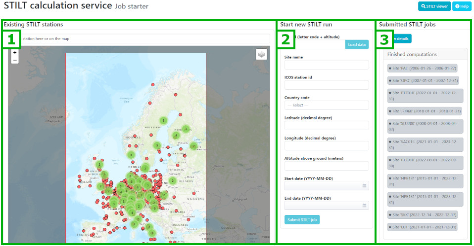
The calculation service consists of three sections, as shown in the screenshot below: 1) the station selection map; 2) the STILT run configuration settings; and 3) the submitted STILT job log.
Step 1: Select the station location
First, you must select the station location from which to calculate footprints. These can be previously defined stations (at existing or new altitudes) or entirely new locations within the boundaries of the footprint model domain.
a) Previously defined stations can be selected from the drop-down list or by locating them on the map. Alternatively, you can type in the name in site id text entry box and click the Load data button to load the predefined coordinates.
b) If you want to start a run for a previously defined location but a new altitude (measurement height), first select the Site id of the existing site and click the Load data button to load the predefined coordinates. Next, change the Site id to include the new altitude (e.g., "HTM015" for a 15m altitude at station HTM). This will unlock the Altitude above ground box, allowing you to enter the new measurement height.
c) For a new station location, you can enter Latitude, Longitude and Altitude above ground in the respective boxes, or you can click on the map to set Latitude and Longitude, then enter the desired Altitude above ground.
For stations in mountainous regions, please see the specific instructions at the end of this page.
Also, please check if computations for a station close by your selected site already exist. With our current model version, simulation results will not be significantly different for stations at less than 10 km distance. Calculations for several sampling heights at tall towers are, of course, still possible.
Define a new, unique Site id following the scheme of a 3-letter code, extended by 3 digits for the altitude above ground in case of several measurement heights. Note that the station should not be located very close to the boundaries of the model domain (34°N–72°N, 14°W–34°E).
Provide a Site name for your new location, which could be the name of the measurement station or a nearby town. Then, select the Country code corresponding to the country in which the new site is located from the drop-down list.
Step 2: Select the time range
Enter the Start date and End date in the respective boxes, or use the calendar tool, available to the right of the entry boxes, to select the dates. Valid dates are highlighted in the calendar tool, starting from 2006-03-01.
Footprints and tracer concentrations will be calculated at 3-hour intervals (00:00, 03:00, 06:00, 09:00, 12:00, 15:00, 18:00, and 21:00 UTC) for each day in the time range.
Note that a calculation for one single day may take up to 24 minutes on a single CPU (or less if all CPUs are available for the job) and waiting time can occur in case of several concurrent calculations.
Step 3: Submit your job
After confirming your information is correct, submit your job by clicking the Submit STILT job button.
Step 4: Check the progress of your computation
You can check the progress of the computation on the dashboard by clicking the Show details button. Your job should show up on the list of running computations, identifiable by the email address you used to log in. Note that you can still delete your submitted job during runtime.
The progress of the computations is indicated by the number of finished time steps (done: progress of total), along with a time estimate (minutes left).
The overall status of the compute server is shown by the number of busy CPUs in relation to the total number of available CPUs, shown at the top of the dashboard.
Step 5: View the results
As soon as the calculations are finished, your job will be moved to the Finished computations list and a View results button will appear. Click on the button to see the visualization in the STILT results viewer. (Please see the STILT results viewer documentation for more details regarding the visualization tool.)
Your new results will now also be available on the list of stations in the STILT viewer.
Note that the job list will be continuously updated and your finished jobs will eventually disappear from the list. Your results will continue to be available in the list of stations in the STILT results viewer.
If you have any questions regarding the STILT calculation service or results views, please contact us at footprint (at) icos-cp.eu
Specific instructions
High mountain stations are often difficult to represent in atmospheric transport model simulations. Therefore, they require a special choice of the Altitude above ground parameter in the computations.
In the model simulations, the Altitude above ground (or measurement height) for a mountain station cannot simply correspond to the height above ground level, as would be the case for a flatland site. This would result in an underestimation of the vertical position in the troposphere, because mountains are not fully resolved by the orography used in the model. On the other hand, placing the station in the simulations at a higher Altitude above ground to offset this underestimation and align with the actual measurement height above sea level would lead to an exaggerated measurement height above ground. This, in turn, would underestimate the interaction between surface fluxes and atmospheric tracer concentration. Currently, we use an expert estimate based on some case studies. Thus, please contact us for help at footprint (at) icos-cp.eu to find an appropriate choice of the Altitude above ground parameter for your mountain site.